Gender Equality Index in the EU

Using ggiraph to recreate an interactive visualization from The Economist.

Exploring Gender Equality in the EU

Purpose

Show a workflow in creating an interactive figure and highlight some data munging tips.

Focus is on:

• Getting data from excel into R with some nice functions etc.
• Interactive charts
• Data viz

Intro

Data from landing page and you can download the excel sheet here.

There are more than 140 indicators that fall into 6 domains and 14 sub-domains.

Description of data ingestion

The data comes in a common format – there is an excel workbook with a readme sheet, then a metadata sheet describing the different variables, then a sheet for the years 2010, 2012, 2015, 2017, 2018 and 2019.

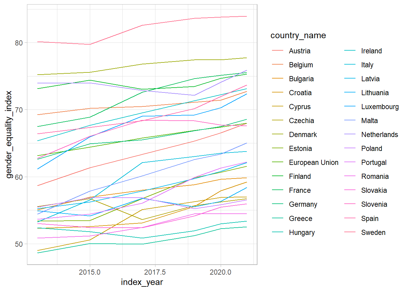
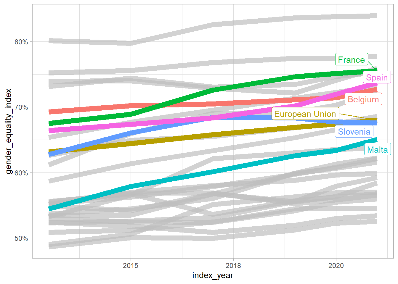
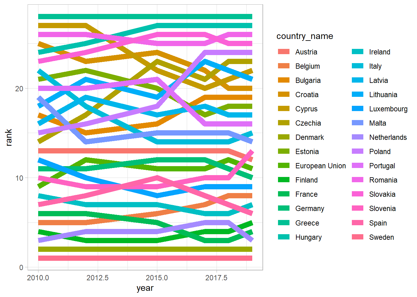
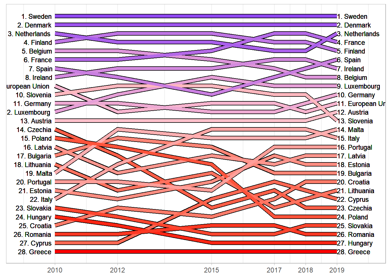
We can make a simple plot of the index changes over time, in relative terms and in absolute terms.

Ingest

Readme sheet

library(tidyverse)

── Attaching packages ─────────────────────────────────────── tidyverse 1.3.2 ──
✔ ggplot2 3.3.6      ✔ purrr   0.3.5 
✔ tibble  3.1.8      ✔ dplyr   1.0.10
✔ tidyr   1.2.1      ✔ stringr 1.4.1 
✔ readr   2.1.3      ✔ forcats 0.5.2 
── Conflicts ────────────────────────────────────────── tidyverse_conflicts() ──
✖ dplyr::filter() masks stats::filter()
✖ dplyr::lag()    masks stats::lag()

library(here)

here() starts at C:/Users/User/Documents/Recon/screencasts

theme_set(theme_light())
df <- readxl::read_excel(here("data/Gender-equality-index.xlsx"))

df %>% 
  knitr::kable()

This excel file is meant to provide users the data needed to calculate the Gender Equality Index
Users must use the data provided in these sheets (one per year), to derive the scores of the Gender Equality Index, by applying the methodology for calculation
Gender Equality Index 2017: Methodological Report | European Institute for Gender Equality (europa.eu)
- Users might find in Index Interface different data for some indicators
- In the Index Interface, EIGE is presenting some of them in a different way
- For instance, the indicator on povery (indicator 8), is considered for calculation as NOT-AT-RISK of POVERTY rate, while in the Index interface, the figures are referred to AT-RISK of POVERTY rate
- The same for the indicators on access to health care, displayed as UNMET NEEDS in the Index interface, and used in a reversed way for calculation.
- As for the indicator of the domain of power, the methodology envisages to use the 3-years average, and the figures in the excel are provided accordingly. In the Index interface, the most updated data (quarterly, biannual, year) are displayed instead.
- The Index Inteface provides the information in the notes and metadata for each indicator

Codebook

The problem is that this is written in a silly way - it’s readable to humans but not to computers

# df <- readxl::read_excel(here("data/Gender-equality-index.xlsx"), sheet = 2, range = )

Data read in process

What we want to do is take the wide dataset from the year tabs and then make them long so that we can collect them together and draw some functions over time.

I should make a graphic of how we go from colours having meaning to columns containing this kind of information. Like a panel on the left where we have a screenshot of the excel sheet - then an arrow - then on the right we have a nice simple grouped dataset on the right.

sheets <- tibble(
  sheet = 3:8,
  year = c(2010, 2012, 2015, 2017, 2018, 2019)
)

get_data <- function(sh) {
  message("Getting data from ", sh)

  df <- readxl::read_excel(here("data/Gender-equality-index.xlsx"), sheet = sh)

  df <- df %>%
    janitor::clean_names() %>%
    pivot_longer(-c(index_year:gender_equality_index))

  df
}

sheets <- sheets %>%
  mutate(data = map(sheet, possibly(get_data, "failed")))

df <- sheets %>%
  unnest(data)

Data augmentation

Country names

We might want to get the English names of a country

df %>% 
  count(country)

We can use the countrycode package:

library(countrycode)

countries <- df %>% 
  distinct(country)

countries <- countries %>% 
  mutate(country_name = countrycode(country, "iso2c", "country.name")) %>% 
  mutate(country_name = case_when(
    country == "EU" ~ "European Union",
    country == "EL" ~ "Greece",
    TRUE ~ country_name
    
    
  ))

df <- df %>% 
  inner_join(countries)

GDP per capita by year

Data from Eurostat:

The indicator is calculated as the ratio of real GDP to the average population of a specific year. GDP measures the value of total final output of goods and services produced by an economy within a certain period of time. It includes goods and services that have markets (or which could have markets) and products which are produced by general government and non-profit institutions. It is a measure of economic activity and is also used as a proxy for the development in a country’s material living standards. However, it is a limited measure of economic welfare. For example, neither does GDP include most unpaid household work nor does GDP take account of negative effects of economic activity, like environmental degradation.

gdp_pc <- readxl::read_excel(here("data/Gender-equality-index_augment_with_gdp_pc.xlsx"), sheet = 3, range = "A9:AS49")

New names:
• `` -> `...3`
• `` -> `...5`
• `` -> `...7`
• `` -> `...9`
• `` -> `...11`
• `` -> `...13`
• `` -> `...15`
• `` -> `...17`
• `` -> `...19`
• `` -> `...21`
• `` -> `...23`
• `` -> `...25`
• `` -> `...27`
• `` -> `...29`
• `` -> `...31`
• `` -> `...33`
• `` -> `...35`
• `` -> `...37`
• `` -> `...39`
• `` -> `...41`
• `` -> `...43`
• `` -> `...45`

cols <- 2*1:22

gdp_pc <- gdp_pc %>% 
  select(1, cols) %>% 
  mutate(across(-TIME, as.numeric)) %>% 
  pivot_longer(-TIME) %>% 
  rename(country_name = TIME) %>% 
  filter(country_name != "GEO (Labels)") %>% 
  mutate(name = parse_number(name)) %>% 
  rename(year = name)

Warning: Using an external vector in selections was deprecated in tidyselect 1.1.0.
ℹ Please use `all_of()` or `any_of()` instead.
  # Was:
  data %>% select(cols)

  # Now:
  data %>% select(all_of(cols))

See <https://tidyselect.r-lib.org/reference/faq-external-vector.html>.

Warning in mask$eval_all_mutate(quo): NAs introduced by coercion

Warning in mask$eval_all_mutate(quo): NAs introduced by coercion

Warning in mask$eval_all_mutate(quo): NAs introduced by coercion

Warning in mask$eval_all_mutate(quo): NAs introduced by coercion

Warning in mask$eval_all_mutate(quo): NAs introduced by coercion

Warning in mask$eval_all_mutate(quo): NAs introduced by coercion

Warning in mask$eval_all_mutate(quo): NAs introduced by coercion

Warning in mask$eval_all_mutate(quo): NAs introduced by coercion

Warning in mask$eval_all_mutate(quo): NAs introduced by coercion

Interactive

library(ggiraph)

f <- gdp_pc %>%
  mutate(
    value_chr = scales::dollar(value),
    tooltip = paste0(country_name, "\n", value_chr, "\n", year)
  ) %>%
  ggplot(aes(x = year, y = value, 
             colour = country_name,
             group = country_name)) +
  geom_point_interactive(aes(tooltip = tooltip), cex = 2) +
  geom_line_interactive() +
  scale_y_continuous(labels = scales::dollar_format()) +
  theme(legend.position = "none") +
  labs(
    x = NULL,
    y = "GDP per capita ",
    caption = "Data from Eurostat"
  )

ggiraph(ggobj = f) %>%
  girafe_options(
    opts_hover(css = girafe_css(
      css = "fill:none;stroke:red;r:5pt;",
      point = "fill:black;stroke:none;"
    )),
    opts_hover_inv(css = girafe_css(
      css = "fill:none;stroke:gray;opacity:.9",
      text = "fill:gray;stroke:none;opacity:.9"
    ))
  )

Warning: Removed 18 rows containing missing values (geom_interactive_point).

Warning: Removed 18 row(s) containing missing values (geom_path).

In prep read in data here

df <- read_rds(here("data/Gender-equality-index.rds"))

df %>% 
  ggplot(aes(index_year, gender_equality_index, colour = country_name)) +
  geom_line()

How can we make the countries more clear?

gghighlight

countries_highlight <- df %>% 
  distinct(country_name) %>% 
  sample_n(6) %>% 
  pull()

df %>%
  mutate(flag = case_when(
    country_name %in% countries_highlight ~ 1,
    TRUE ~ 0
  )) %>%
  ggplot(aes(index_year, gender_equality_index, colour = country_name)) +
  geom_line(size = 3) +
  gghighlight::gghighlight(flag == 1) +
  scale_x_continuous(labels = scales::number_format(accuracy = 1, big.mark = "")) +
  scale_y_continuous(labels = scales::percent_format(scale = 1))

Warning: Tried to calculate with group_by(), but the calculation failed.
Falling back to ungrouped filter operation...

label_key: country_name

Recreate a nice ranking change?

df_rank <- df %>%
  select(reference_year_main, country_name, gender_equality_index) %>%
  distinct()

df_rank <- df_rank %>%
  group_by(reference_year_main) %>%
  mutate(rank = rank(desc(gender_equality_index), ties.method = "average")) %>%
  ungroup() %>%
  rename(year = reference_year_main)

df_rank %>%
  ggplot(aes(year, rank, color = country_name)) +
  geom_line(size = 3)

What elements do we need?

• Labels on left and right that include rank and country name
• Colour scale that goes from blue to red based on ranking at end of period
• Interactivity with ggiraph probably.

Is there a better way to do this?

labels_left <- df_rank %>% 
  filter(year == min(year)) %>% 
  mutate(left_rank = rank) %>% 
  select(country_name, left_rank)

labels_right <- df_rank %>% 
  filter(year == max(year)) %>% 
  mutate(right_rank = rank) %>% 
  select(country_name, right_rank)

df_rank <- df_rank %>% 
  inner_join(labels_left) %>% 
  inner_join(labels_right)

Joining, by = "country_name"
Joining, by = "country_name"

df_rank %>%
  ggplot(aes(year, rank, color = right_rank, group = country_name)) +
  geom_line(size = 2.8, aes(year, rank, group = country_name), colour = "black") +
  geom_line(size = 2) +
  geom_text(aes(
    x = 2010, y = left_rank,
    label = paste0(left_rank, ". ", country_name)
  ),
  colour = "black",
  hjust = 1.1,
  cex = 3
  ) +
  geom_text(aes(
    x = 2019, y = right_rank,
    label = paste0(right_rank, ". ", country_name)
  ),
  colour = "black",
  hjust = 0,
  cex = 3
  ) +
  scale_y_reverse() +
  scale_color_gradient2(
    low = "blue", high = "red",
    mid = "pink",
    midpoint = 12
  ) +
  scale_x_continuous(breaks = c(2010, 2012, 2015, 2017, 2018, 2019)) +
  coord_cartesian(xlim = c(2009, 2020)) +
  theme(
    legend.position = "none",
    panel.grid.major.y = element_blank(),
    panel.grid.minor.y = element_blank(),
    axis.ticks.y = element_blank(),
    axis.text.y = element_blank()
  ) +
  labs(
    x = NULL,
    y = NULL
  ) 

Interactivity

library(ggiraph)

g <- df_rank %>%
  ggplot(aes(year, rank, color = right_rank, group = country_name, tooltip = country_name)) +
  geom_line(size = 2.8, aes(year, rank, group = country_name), colour = "black") +
  geom_line_interactive(size = 2, aes(data_id = country_name)) +
  geom_text_interactive(aes(
    x = 2010, y = left_rank,
    label = paste0(left_rank, ". ", country_name),
    data_id = country_name
  ),
  colour = "black", hjust = 1.1, cex = 3
  ) +
  geom_text_interactive(aes(
    x = 2019, y = right_rank,
    label = paste0(right_rank, ". ", country_name),
    data_id = country_name
  ),
  colour = "black", hjust = 0, cex = 3
  ) +
  scale_y_reverse() +
  scale_color_gradient2(
    low = "blue", high = "red", mid = "pink",
    midpoint = 14
  ) +
  scale_x_continuous(breaks = c(2010, 2012, 2015, 2017, 2018, 2019)) +
  coord_cartesian(xlim = c(2008, 2021)) +
  theme(
    legend.position = "none",
    panel.grid.major.y = element_blank(),
    panel.grid.minor.y = element_blank(),
    axis.ticks.y = element_blank(),
    axis.text.y = element_blank()
  ) +
  labs(
    x = NULL,
    y = NULL
  )

ggiraph(ggobj = g) %>%
  girafe_options(
    opts_hover(css = girafe_css(
      css = "fill:none;stroke:red;r:5pt;",
      text = "fill:black;stroke:none;"
    )),
    opts_hover_inv(css = girafe_css(
      css = "fill:none;stroke:gray;opacity:.9",
      text = "fill:gray;stroke:none;opacity:.9"
    ))
  )

Yay! It works! Have a look at Hungary falling right to the bottom.

Great. I hope that was useful.