Purpose
Translate the code from session 3 to R.
Read in data
-- Attaching packages --------------------------------------- tidyverse 1.3.1 --
v ggplot2 3.3.5     v purrr   0.3.4
v tibble  3.1.6     v dplyr   1.0.7
v tidyr   1.1.4     v stringr 1.4.0
v readr   2.1.1     v forcats 0.5.1
Warning: package 'tibble' was built under R version 4.1.2
Warning: package 'readr' was built under R version 4.1.2
-- Conflicts ------------------------------------------ tidyverse_conflicts() --
x dplyr::filter() masks stats::filter()
x dplyr::lag()    masks stats::lag()
theme_set (theme_light ())<- readxl:: read_excel (here:: here ("course-content/Class 3/Kelly and O Grada (2013).xlsx" ),range = "A1:F256" )# tidy up variable names <- df %>% :: clean_names ()
Changes
<- df %>% mutate (real_gdp_pc = real_gdp / population,real_agricultural_output_pc = real_agricultural_output / population,# create logs with prefix ln_ across (c (crude_death_rate: real_wage, contains ("_pc" )), log, .names = "ln_{.col}" ),# create differences with prefix d_ across (c (contains ("ln_" )), ~ . - lag (., 1 ), .names = "d_{.col}" ))
Now making the lags of the differenced variables: I don’t love this for loop - but I don’t know a better way yet. Perhaps using the recipes package?
for (i in 1 : 4 ) {message ("making d_ for " , i)<- df %>% mutate (across (starts_with ("d_ln" ), ~ lag (., i), .names = paste0 ("l" , i, "_{.col}" )))
What about using the recipes package?
# library(recipes)
#
# rec <- recipe(d_ln_crude_death_rate ~ ., data = df) %>%
#   step_log(c(crude_death_rate:real_wage, contains("_pc")), id = rand_id(prefix = "ln_"))
#
#
# rec %>% prep() %>% bake(new_data = NULL)
Data summary
Name
Piped data
Number of rows
255
Number of columns
32
_______________________
Column type frequency:
numeric
32
________________________
Group variables
None
Variable type: numeric
year
0
1.00
1672.00
73.76
1545.00
1608.50
1672.00
1735.50
1799.00
▇▇▇▇▇
crude_death_rate
0
1.00
27.50
4.60
19.20
24.90
26.80
29.00
53.90
▇▇▁▁▁
real_wage
0
1.00
72.57
11.34
50.55
65.22
71.05
77.13
114.01
▃▇▃▁▁
real_agricultural_output
0
1.00
106.56
40.04
41.51
77.58
95.74
128.49
216.93
▅▇▃▂▂
real_gdp
0
1.00
92.79
45.63
32.46
56.77
79.00
119.32
226.06
▇▅▃▂▁
population
0
1.00
99.86
24.78
55.98
85.01
100.00
110.00
170.01
▅▇▆▂▁
real_gdp_pc
0
1.00
0.88
0.23
0.52
0.69
0.80
1.09
1.34
▇▇▃▆▅
real_agricultural_output_pc
0
1.00
1.05
0.19
0.59
0.90
1.06
1.19
1.54
▂▆▇▆▁
ln_crude_death_rate
0
1.00
3.30
0.15
2.95
3.21
3.29
3.37
3.99
▂▇▂▁▁
ln_real_wage
0
1.00
4.27
0.15
3.92
4.18
4.26
4.35
4.74
▂▇▇▂▁
ln_real_gdp_pc
0
1.00
-0.16
0.26
-0.64
-0.38
-0.23
0.08
0.29
▃▇▃▅▆
ln_real_agricultural_output_pc
0
1.00
0.03
0.19
-0.53
-0.10
0.06
0.18
0.43
▁▃▆▇▃
d_ln_crude_death_rate
1
1.00
0.00
0.14
-0.50
-0.07
0.00
0.06
0.55
▁▂▇▁▁
d_ln_real_wage
1
1.00
0.00
0.11
-0.35
-0.06
0.00
0.07
0.42
▁▃▇▂▁
d_ln_real_gdp_pc
1
1.00
0.00
0.08
-0.31
-0.04
0.00
0.04
0.26
▁▁▇▃▁
d_ln_real_agricultural_output_pc
1
1.00
0.00
0.16
-0.60
-0.10
-0.01
0.10
0.46
▁▁▇▅▁
l1_d_ln_crude_death_rate
2
0.99
0.00
0.14
-0.50
-0.07
0.00
0.06
0.55
▁▂▇▁▁
l1_d_ln_real_wage
2
0.99
0.00
0.11
-0.35
-0.06
0.00
0.07
0.42
▁▃▇▂▁
l1_d_ln_real_gdp_pc
2
0.99
0.00
0.08
-0.31
-0.04
0.00
0.04
0.26
▁▁▇▃▁
l1_d_ln_real_agricultural_output_pc
2
0.99
0.00
0.16
-0.60
-0.10
0.00
0.10
0.46
▁▁▇▅▁
l2_d_ln_crude_death_rate
3
0.99
0.00
0.14
-0.50
-0.07
0.00
0.06
0.55
▁▂▇▁▁
l2_d_ln_real_wage
3
0.99
0.00
0.11
-0.35
-0.06
0.00
0.07
0.42
▁▃▇▂▁
l2_d_ln_real_gdp_pc
3
0.99
0.00
0.08
-0.31
-0.04
0.00
0.04
0.26
▁▁▇▃▁
l2_d_ln_real_agricultural_output_pc
3
0.99
0.00
0.16
-0.60
-0.10
-0.01
0.10
0.46
▁▁▇▅▁
l3_d_ln_crude_death_rate
4
0.98
0.00
0.14
-0.50
-0.07
0.00
0.06
0.55
▁▂▇▁▁
l3_d_ln_real_wage
4
0.98
0.00
0.11
-0.35
-0.06
0.00
0.07
0.42
▁▃▇▂▁
l3_d_ln_real_gdp_pc
4
0.98
0.00
0.08
-0.31
-0.04
0.00
0.05
0.26
▁▁▇▃▁
l3_d_ln_real_agricultural_output_pc
4
0.98
0.00
0.16
-0.60
-0.10
0.00
0.10
0.46
▁▁▇▅▁
l4_d_ln_crude_death_rate
5
0.98
0.00
0.14
-0.50
-0.07
0.00
0.06
0.55
▁▂▇▁▁
l4_d_ln_real_wage
5
0.98
0.00
0.11
-0.35
-0.06
0.00
0.07
0.42
▁▃▇▂▁
l4_d_ln_real_gdp_pc
5
0.98
0.00
0.08
-0.31
-0.04
0.00
0.05
0.26
▁▁▇▃▁
l4_d_ln_real_agricultural_output_pc
5
0.98
0.00
0.16
-0.60
-0.11
0.00
0.10
0.46
▁▁▇▅▁
(Approximately) Reproduce Table 6
What are we doing?
3 sets of regressions
Change in crude death rate is dependent var
5 time periods
We should use the many models approach from R4DS because we’re doing similar regressions on different sections of the data frame.
<- tibble (left = c (1546 ,1600 ,1650 ,1700 ,1750 %>% mutate (right = case_when (== 1546 ~ 1599 ,TRUE ~ left + 49 period = row_number ()<- periods %>% group_by (period) %>% mutate (year = paste0 (left: right, collapse = ", " )) %>% ungroup () %>% separate_rows (year, sep = ", " , convert = T) %>% :: select (- c (left, right))<- df %>% inner_join (periods)<- df_by_period %>% filter (! is.na (period)) %>% group_by (period) %>% nest ()
Function to do regression
<- function (df, vars){<- df %>% :: select (d_ln_crude_death_rate, vars)lm (d_ln_crude_death_rate ~ ., data = df_temp)
First regression model
<- df_by_period %>% mutate (model = map (data, ~ reg_model (df = .,vars = c (contains ("_d_ln_real_wage" ), contains ("d_ln_crude_death_rate" )))))
Note: Using an external vector in selections is ambiguous.
i Use `all_of(vars)` instead of `vars` to silence this message.
i See <https://tidyselect.r-lib.org/reference/faq-external-vector.html>.
This message is displayed once per session.
What do the regression outputs look like?
%>% mutate (summary = map (model, summary)) %>% pull (summary)
[[1]]

Call:
lm(formula = d_ln_crude_death_rate ~ ., data = df_temp)

Residuals:
     Min       1Q   Median       3Q      Max
-0.29614 -0.06895 -0.00877  0.09223  0.37833

Coefficients:
                         Estimate Std. Error t value Pr(>|t|)
(Intercept)              -0.01790    0.02110  -0.848 0.401214
l1_d_ln_real_wage        -0.38635    0.18148  -2.129 0.039318 *
l2_d_ln_real_wage        -0.74798    0.19933  -3.752 0.000543 ***
l3_d_ln_real_wage        -0.28785    0.20773  -1.386 0.173331
l4_d_ln_real_wage        -0.41609    0.18345  -2.268 0.028655 *
l1_d_ln_crude_death_rate -0.21795    0.14858  -1.467 0.150030
l2_d_ln_crude_death_rate -0.39873    0.14154  -2.817 0.007422 **
l3_d_ln_crude_death_rate -0.46959    0.12402  -3.786 0.000491 ***
l4_d_ln_crude_death_rate -0.02081    0.14534  -0.143 0.886845
---
Signif. codes:  0 '***' 0.001 '**' 0.01 '*' 0.05 '.' 0.1 ' ' 1

Residual standard error: 0.1455 on 41 degrees of freedom
  (4 observations deleted due to missingness)
Multiple R-squared:  0.459, Adjusted R-squared:  0.3534
F-statistic: 4.348 on 8 and 41 DF,  p-value: 0.0007355


[[2]]

Call:
lm(formula = d_ln_crude_death_rate ~ ., data = df_temp)

Residuals:
     Min       1Q   Median       3Q      Max
-0.23308 -0.08450 -0.01951  0.04716  0.40095

Coefficients:
                          Estimate Std. Error t value Pr(>|t|)
(Intercept)              -0.003599   0.019679  -0.183  0.85579
l1_d_ln_real_wage        -0.669875   0.209793  -3.193  0.00270 **
l2_d_ln_real_wage        -0.099300   0.236031  -0.421  0.67617
l3_d_ln_real_wage        -0.110009   0.223259  -0.493  0.62482
l4_d_ln_real_wage        -0.136204   0.217440  -0.626  0.53453
l1_d_ln_crude_death_rate -0.350978   0.153727  -2.283  0.02768 *
l2_d_ln_crude_death_rate -0.206345   0.142099  -1.452  0.15408
l3_d_ln_crude_death_rate -0.413009   0.138295  -2.986  0.00475 **
l4_d_ln_crude_death_rate -0.193783   0.131117  -1.478  0.14706
---
Signif. codes:  0 '***' 0.001 '**' 0.01 '*' 0.05 '.' 0.1 ' ' 1

Residual standard error: 0.1387 on 41 degrees of freedom
Multiple R-squared:  0.4041,    Adjusted R-squared:  0.2879
F-statistic: 3.476 on 8 and 41 DF,  p-value: 0.003795


[[3]]

Call:
lm(formula = d_ln_crude_death_rate ~ ., data = df_temp)

Residuals:
     Min       1Q   Median       3Q      Max
-0.24972 -0.07429 -0.01702  0.04027  0.42011

Coefficients:
                          Estimate Std. Error t value Pr(>|t|)
(Intercept)               0.007543   0.018804   0.401  0.69041
l1_d_ln_real_wage         0.226045   0.161795   1.397  0.16990
l2_d_ln_real_wage         0.110585   0.168958   0.655  0.51644
l3_d_ln_real_wage         0.225356   0.167501   1.345  0.18589
l4_d_ln_real_wage         0.132567   0.160166   0.828  0.41264
l1_d_ln_crude_death_rate -0.420488   0.158959  -2.645  0.01152 *
l2_d_ln_crude_death_rate -0.471103   0.158121  -2.979  0.00484 **
l3_d_ln_crude_death_rate -0.331769   0.163544  -2.029  0.04903 *
l4_d_ln_crude_death_rate  0.011955   0.157786   0.076  0.93997
---
Signif. codes:  0 '***' 0.001 '**' 0.01 '*' 0.05 '.' 0.1 ' ' 1

Residual standard error: 0.1321 on 41 degrees of freedom
Multiple R-squared:  0.3326,    Adjusted R-squared:  0.2024
F-statistic: 2.555 on 8 and 41 DF,  p-value: 0.02333


[[4]]

Call:
lm(formula = d_ln_crude_death_rate ~ ., data = df_temp)

Residuals:
      Min        1Q    Median        3Q       Max
-0.203460 -0.049068  0.003584  0.041974  0.199835

Coefficients:
                          Estimate Std. Error t value Pr(>|t|)
(Intercept)               0.004618   0.013619   0.339   0.7363
l1_d_ln_real_wage        -0.428433   0.183713  -2.332   0.0247 *
l2_d_ln_real_wage        -0.164349   0.184840  -0.889   0.3791
l3_d_ln_real_wage        -0.250078   0.180839  -1.383   0.1742
l4_d_ln_real_wage         0.084341   0.183335   0.460   0.6479
l1_d_ln_crude_death_rate -0.032322   0.155396  -0.208   0.8363
l2_d_ln_crude_death_rate -0.229270   0.145303  -1.578   0.1223
l3_d_ln_crude_death_rate -0.256747   0.145251  -1.768   0.0846 .
l4_d_ln_crude_death_rate  0.085290   0.153253   0.557   0.5809
---
Signif. codes:  0 '***' 0.001 '**' 0.01 '*' 0.05 '.' 0.1 ' ' 1

Residual standard error: 0.09458 on 41 degrees of freedom
Multiple R-squared:  0.3128,    Adjusted R-squared:  0.1787
F-statistic: 2.333 on 8 and 41 DF,  p-value: 0.03637


[[5]]

Call:
lm(formula = d_ln_crude_death_rate ~ ., data = df_temp)

Residuals:
      Min        1Q    Median        3Q       Max
-0.108223 -0.031518 -0.005504  0.029754  0.093847

Coefficients:
                          Estimate Std. Error t value Pr(>|t|)
(Intercept)              -0.000632   0.007377  -0.086  0.93214
l1_d_ln_real_wage         0.180114   0.153033   1.177  0.24600
l2_d_ln_real_wage         0.193466   0.154924   1.249  0.21883
l3_d_ln_real_wage         0.357952   0.154271   2.320  0.02538 *
l4_d_ln_real_wage         0.460454   0.164170   2.805  0.00766 **
l1_d_ln_crude_death_rate -0.473955   0.141671  -3.345  0.00177 **
l2_d_ln_crude_death_rate -0.281857   0.142263  -1.981  0.05430 .
l3_d_ln_crude_death_rate -0.210367   0.143704  -1.464  0.15085
l4_d_ln_crude_death_rate  0.225747   0.145367   1.553  0.12812
---
Signif. codes:  0 '***' 0.001 '**' 0.01 '*' 0.05 '.' 0.1 ' ' 1

Residual standard error: 0.05174 on 41 degrees of freedom
Multiple R-squared:  0.4289,    Adjusted R-squared:  0.3175
F-statistic:  3.85 on 8 and 41 DF,  p-value: 0.001858
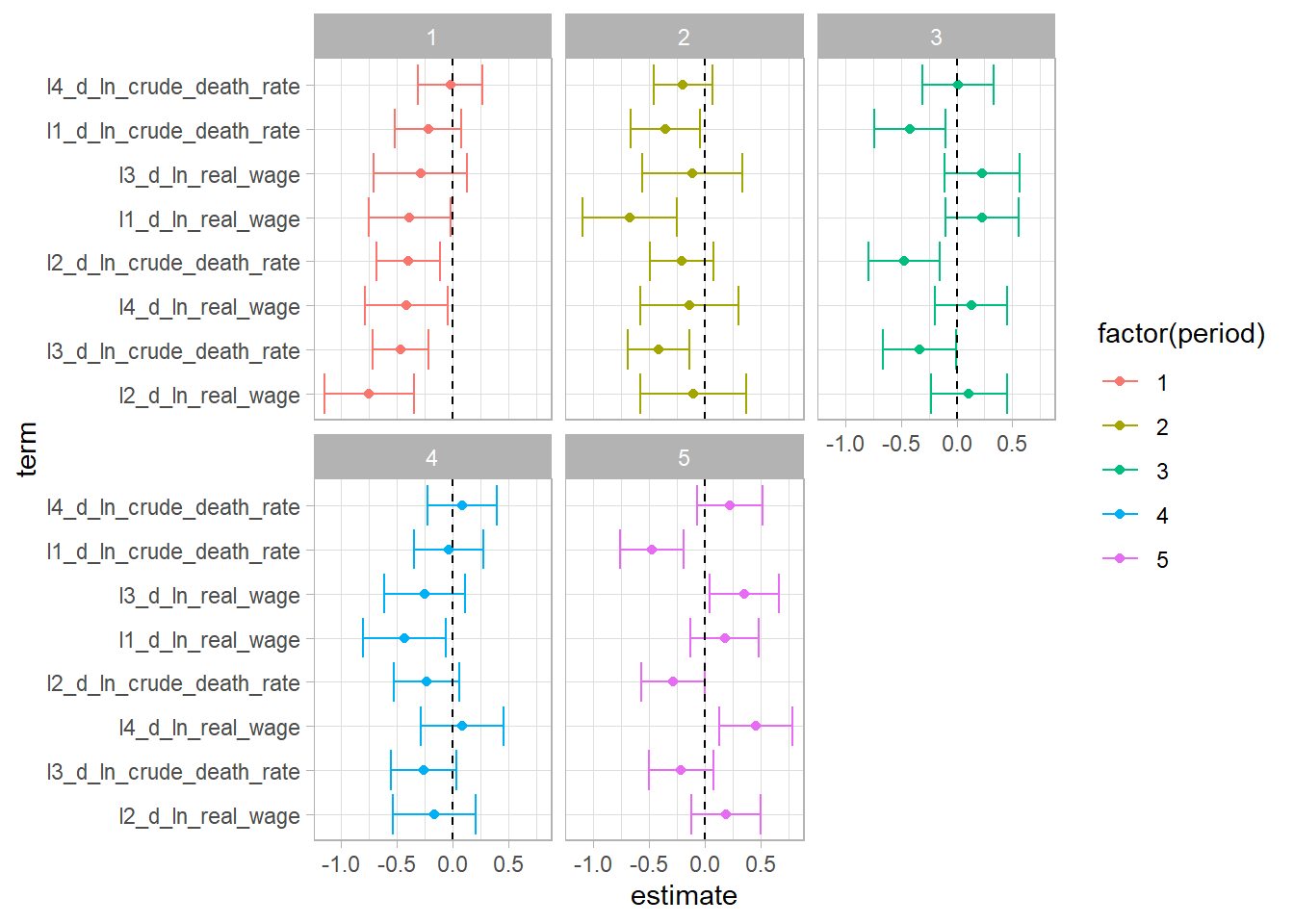
How can we format these better??
%>% mutate (tidy = map (model, ~ broom:: tidy (., conf.int = T))) %>% unnest (tidy) %>% filter (term != "(Intercept)" ) %>% mutate (term = fct_reorder (term, estimate)) %>% ggplot (aes (estimate, term, colour = factor (period))) + geom_point () + geom_errorbarh (aes (xmin = conf.low, xmax = conf.high)) + facet_wrap (~ period) + geom_vline (xintercept = 0 , lty = 2 )
# df_by_period_reg %>%
#   mutate(reg = map(model, gtsummary::tbl_regression)) %>%
#   pull(reg)
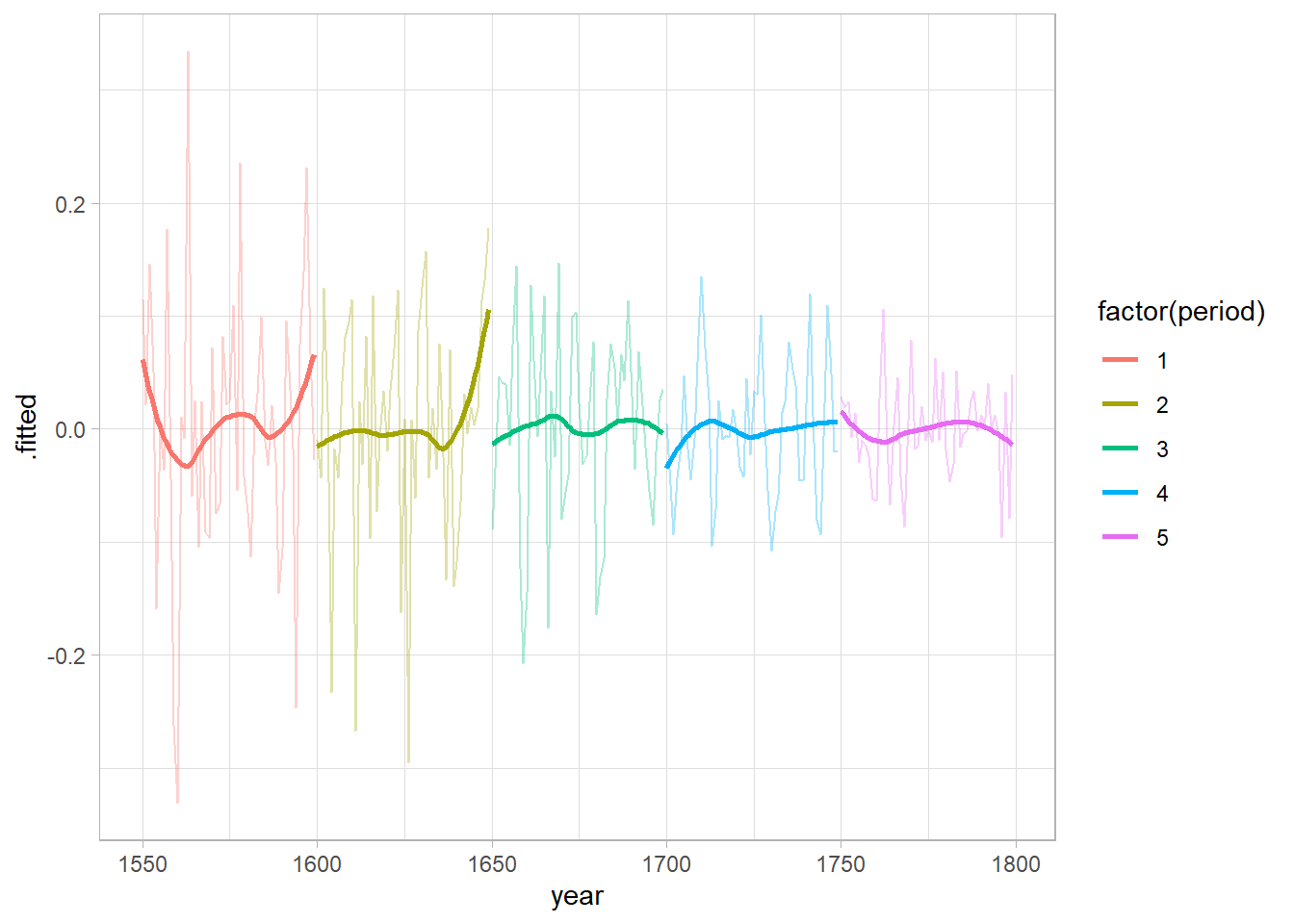
%>% mutate (augment = map (model, broom:: augment)) %>% unnest (augment) %>% # remove the first four NA years because of the lags (4 lags) bind_cols (periods %>% tail (250 ) %>% dplyr:: select (- period)) %>% ggplot (aes (year, .fitted, group = period, colour = factor (period))) + geom_line (alpha = 1 / 3 ) + geom_smooth (se = FALSE )
`geom_smooth()` using method = 'loess' and formula 'y ~ x'
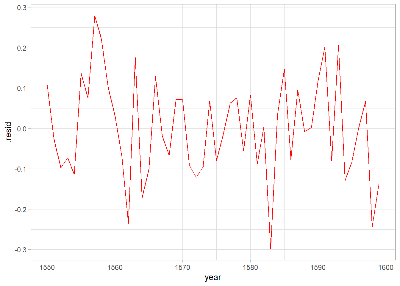
Evaluate the residuals
Regression:
dependent variable: first difference of logged crude death rate
independent variables: lags 1 through 4 of first diff of ln crude death rate and first diff of ln real gdp per capita
# reg d.LnCrudeDeathRate L(1/4)d.LnCrudeDeathRate L(0/4)d.LnRealGDPpc if tin(1546,1599)
# predict Residuals if tin(1546,1599), res /* generate the residuals as a new variable */
# tsline Residuals if tin(1546,1599) /* plot the residuals */
Warning: package 'gtsummary' was built under R version 4.1.2
<- df %>% filter (between (year, 1546 , 1599 )) %>% :: select (c (contains ("d_ln_real_gdp_pc" ),contains ("d_ln_crude_death_rate" )%>% lm (d_ln_crude_death_rate ~ ., data = .)%>% tbl_regression () %>% add_significance_stars ()
Characteristic Beta SE
d_ln_real_gdp_pc
0.33
0.236 l1_d_ln_real_gdp_pc
-0.59*
0.260 l2_d_ln_real_gdp_pc
-0.85**
0.300 l3_d_ln_real_gdp_pc
-0.84*
0.325 l4_d_ln_real_gdp_pc
-0.02
0.309 l1_d_ln_crude_death_rate
-0.30
0.157 l2_d_ln_crude_death_rate
-0.16
0.142 l3_d_ln_crude_death_rate
-0.30*
0.133 l4_d_ln_crude_death_rate
-0.03
0.139
Plot the residuals
<- reg_1 %>% :: augment () %>% bind_cols (periods %>% :: select (year) %>% slice (5L: 54L))%>% ggplot (aes (year, .resid)) + geom_line (colour = "red" )
Dickey fuller tests
Warning: package 'vars' was built under R version 4.1.3
Loading required package: MASS
Attaching package: 'MASS'
The following object is masked from 'package:gtsummary':

    select
The following object is masked from 'package:dplyr':

    select
Loading required package: strucchange
Warning: package 'strucchange' was built under R version 4.1.3
Loading required package: zoo
Warning: package 'zoo' was built under R version 4.1.3
The following objects are masked from 'package:base':

    as.Date, as.Date.numeric
Loading required package: sandwich
Warning: package 'sandwich' was built under R version 4.1.3
Attaching package: 'strucchange'
The following object is masked from 'package:stringr':

    boundary
Loading required package: urca
Loading required package: lmtest
Warning: package 'lmtest' was built under R version 4.1.3
<- ur.df (reg_1_augmented$ .resid, type = "trend" )%>% summary ()
###############################################
# Augmented Dickey-Fuller Test Unit Root Test #
###############################################

Test regression trend


Call:
lm(formula = z.diff ~ z.lag.1 + 1 + tt + z.diff.lag)

Residuals:
      Min        1Q    Median        3Q       Max
-0.284507 -0.087212  0.006262  0.081510  0.254474

Coefficients:
              Estimate Std. Error t value Pr(>|t|)
(Intercept)  0.0219943  0.0395612   0.556 0.581057
z.lag.1     -0.9218949  0.2198818  -4.193 0.000131 ***
tt          -0.0009444  0.0013623  -0.693 0.491768
z.diff.lag  -0.0474320  0.1569519  -0.302 0.763918
---
Signif. codes:  0 '***' 0.001 '**' 0.01 '*' 0.05 '.' 0.1 ' ' 1

Residual standard error: 0.1305 on 44 degrees of freedom
Multiple R-squared:  0.4827,    Adjusted R-squared:  0.4474
F-statistic: 13.68 on 3 and 44 DF,  p-value: 1.93e-06


Value of test-statistic is: -4.1927 5.9638 8.8931

Critical values for test statistics:
      1pct  5pct 10pct
tau3 -4.15 -3.50 -3.18
phi2  7.02  5.13  4.31
phi3  9.31  6.73  5.61
<- ur.df (reg_1_augmented$ .resid, type = "none" )%>% summary ()
###############################################
# Augmented Dickey-Fuller Test Unit Root Test #
###############################################

Test regression none


Call:
lm(formula = z.diff ~ z.lag.1 - 1 + z.diff.lag)

Residuals:
      Min        1Q    Median        3Q       Max
-0.293606 -0.089575 -0.004895  0.078174  0.269227

Coefficients:
           Estimate Std. Error t value Pr(>|t|)
z.lag.1    -0.91447    0.21562  -4.241 0.000106 ***
z.diff.lag -0.04852    0.15399  -0.315 0.754134
---
Signif. codes:  0 '***' 0.001 '**' 0.01 '*' 0.05 '.' 0.1 ' ' 1

Residual standard error: 0.1283 on 46 degrees of freedom
Multiple R-squared:  0.477, Adjusted R-squared:  0.4542
F-statistic: 20.97 on 2 and 46 DF,  p-value: 3.36e-07


Value of test-statistic is: -4.2411

Critical values for test statistics:
      1pct  5pct 10pct
tau1 -2.62 -1.95 -1.61
<- ur.df (reg_1_augmented$ .resid, type = "drift" )%>% summary ()
###############################################
# Augmented Dickey-Fuller Test Unit Root Test #
###############################################

Test regression drift


Call:
lm(formula = z.diff ~ z.lag.1 + 1 + z.diff.lag)

Residuals:
     Min       1Q   Median       3Q      Max
-0.29139 -0.08746 -0.00280  0.08031  0.27117

Coefficients:
             Estimate Std. Error t value Pr(>|t|)
(Intercept) -0.002111   0.018765  -0.112 0.910946
z.lag.1     -0.913223   0.218255  -4.184 0.000131 ***
z.diff.lag  -0.049675   0.156010  -0.318 0.751649
---
Signif. codes:  0 '***' 0.001 '**' 0.01 '*' 0.05 '.' 0.1 ' ' 1

Residual standard error: 0.1297 on 45 degrees of freedom
Multiple R-squared:  0.477, Adjusted R-squared:  0.4538
F-statistic: 20.52 on 2 and 45 DF,  p-value: 4.634e-07


Value of test-statistic is: -4.1842 8.807

Critical values for test statistics:
      1pct  5pct 10pct
tau2 -3.58 -2.93 -2.60
phi1  7.06  4.86  3.94
Breusch–Pagan Test to Check Heteroscedasticity
# library(plm)
#
# df_bp <- df %>%
#   dplyr::filter(dplyr::between(year, 1546, 1599)) %>%
#   dplyr::select(c(
#     contains("d_ln_real_gdp_pc"),
#     contains("d_ln_crude_death_rate")
#   )) %>% na.omit()
#
# df_bp %>% colnames() %>% paste0(., collapse = " + ")
#
# plmtest(d_ln_real_gdp_pc ~ l1_d_ln_real_gdp_pc + l2_d_ln_real_gdp_pc + l3_d_ln_real_gdp_pc + l4_d_ln_real_gdp_pc + d_ln_crude_death_rate + l1_d_ln_crude_death_rate + l2_d_ln_crude_death_rate + l3_d_ln_crude_death_rate + l4_d_ln_crude_death_rate,
#         data = df_bp,
#         type = "bp")